Transformation task best practice
When configuring and executing your transformation tasks, we recommend the following best practice advice:
For a stable and optimized data pipeline, we recommend executing delta transformations in your data model. Delta transformations process only the new or updated records from your data, rather than the full load each time. When configuring delta transformations, you need to set the primary keys for each table, allowing a MERGE to be performed.
For a performant and stable data pipeline only the newly extracted records should be transformed.
Let’s say you have fully loaded the case table, i.e. SalesOrderItems, and run transformations to build your Case table based on VBAP. The subsequent refreshes of VBAP, i.e. delta extractions, bring the new records from the source system. Of course, these new records should be propagated to the Case table as well so that they are reflected in the user-facing analysis. There are two ways in which you can do this:
Drop and recreate the Case table (initialize it).
Process only the new records, i.e. execute a delta transformation.
Option 1 ensures data integrity and is relatively easier to implement. However it is not performant, especially as the data size grows. This is not the recommended approach.
Option 2 requires more implementation effort because a MERGE should be done based on the primary keys. In this option, only the incoming date is processed which ensured the maximal performance. We recommend choosing this option.
The sections below explain delta transformations in more detail.
Storing the Delta in a Staging Table
To be able to process the delta we need to isolate it. This is done by pushing the extracted delta into a separate staging table. So if you are extracting BKPF, the new delta is pushed not only to the BKPF, but also in a staging table called _CELONIS_TMP_BKPF_NEW_DATA. This enables the user to later access this data and use it for transformations.
Accessing the Delta from the Staging Table
After the extraction is complete, transformations should access the delta from the staging table. Theoretically we can select directly from the table _CELONIS_STAGING_BKPF, but this will make the SQL script unusable for full transformations, i.e. when we want to select from the source BKPF and recreate the data model.
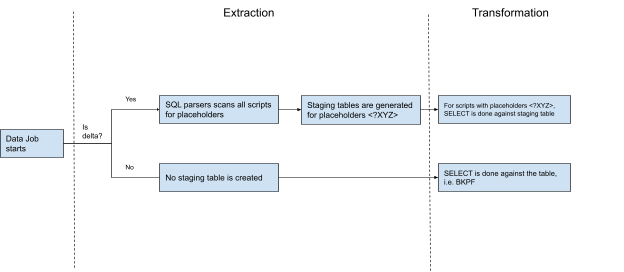
To solve this we have introduced the concept of the placeholder. So in the SQL instead of referencing to BKPF, the select is done against <$BKPF>. Depending on the execution type - delta vs full - this placeholder is dynamically translated into a table name.
For full execution it is replaced by BKPF, so the query becomes SELECT * FROM BKPF.
For delta execution it is replaced by _CELONIS_TMP_BKPF_NEW_DATA, o the query becomes SELECT * FROM _CELONIS_TMP_BKPF_NEW_DATA.
This placeholder is also very important because based on that the extractor decides for which tables to generate a staging table. See the next section for more details.
How is the Staging Table Generated?
The delta should be isolated only for the tables which are a source for transformations, i.e. against which a SELECT statement is written. So if you are extracting 4 tables, but only BKPF acts as source for select, then we need to capture the delta only for this table.
To reduce the manual steps, this step, i.e. identifying which tables to generate a staging table for, has been automated. Before running the extraction, the “SQL parsers” scans all the SQL scripts in the given Data Job. Whenever it spots placeholder, e.g. <$BKPF>, it also marks this table as eligible for generating a staging table for. If you have 10 tables in the extraction, but only one SELECT statement against a placeholder, i.e. <$BKPF>, then only one staging table will be generated - _CELONIS_STAGING_BKPF.
 |
Staging Table Clean Up
After a successful run, the staging table is cleaned up. This is to ensure that during the next execution we don’t reprocess the same records. However, it is important to note that not all records are cleaned up. For referential integrity we keep some of them to be reprocessed two times. This is mostly to address dependencies between tables, i.e. when there is a JOIN between them. In case a record in a dependent table arrives late, we might want to reprocess the records in a staging table, so that the JOIN works properly. One example is VBAK and VBAP. When building the case table based on VBAP, we fetch a lot of information from VBAK via a join. A VBAP record is extracted, but its header record might be missing due to timing issues. In that case we would like to reprocess the VBAP record again during the next delta run to ensure that VBAK has already been extracted.
How the SQL should be written
Delta transformations requires to:
persist the transformed data
merge the incoming data rather than drop/recreate
The SQL scripts should implement these two requirements. The transformed data should be persisted. So if you are doing some transformations based on BSID, then you should create a target table which will store those calculations. Here is an example:
DROP TABLE IF EXISTS BSID_CALCULATED;  CREATE TABLE BSID_CALCULATED(
MANDT varchar(12),
BUKRS varchar(16),
BELNR varchar(40),
GJAHR varchar(16),
BUZEI varchar(12),
WRBTR_CONVERTED float,
SKFBT_CONVERTED float,
WSKTO_CONVERTED float,
BUKRS_TEXT varchar(100),
ZTERM_MD varchar(16),
ZTAGG_MD varchar(8),
ZDART_MD varchar(4),
ZFAEL_MD varchar(8),
ZMONA_MD varchar(8),
ZTAG1_MD varchar(12),
ZPRZ1_MD float,
ZTAG2_MD varchar(12),
ZPRZ2_MD float,
ZTAG3_MD varchar(12));
What we do here is to create a “calculation” table for BSID, where we will store the transformed fields. Note that we don’t store the whole BSID, and only the calculated fields and the Primary Keys. This is to reduce the impact on APC. Primary Keys will be used later to unify the BSID and the transformed values in a view.
As a next step the incoming delta data should be merged to this persisted table. One way to merge is to simply remove the records from the transformed table, and then insert them again. Here is an example on how to implement the deletion for the table BSID.
DELETE FROM "BSID_CALCULATED"
WHERE EXISTS (SELECT 1 FROM <$BSID> as NEW_DATA WHERE AR_BSID_STAGING.MANDT = NEW_DATA.MANDT AND AR_BSID_STAGING.BUKRS = NEW_DATA.BUKRS AND AR_BSID_STAGING.BELNR = NEW_DATA.BELNR AND AR_BSID_STAGING.GJAHR = NEW_DATA.GJAHR AND AR_BSID_STAGING.BUZEI = NEW_DATA.BUZEI );
We basically select all the records from the BSID Staging (via placeholder <$BSID>), and then remove all the matches from the target table, i.e. BSID_CALCULATED.
And then we insert our calculations into the BSID_CALCULATED.
INSERT INTO "BSID_CALCULATED"
SELECT BSID.MANDT ,BSID.BUKRS ,BSID.BELNR ,BSID.GJAHR ,BSID.BUZEI ……… some query ……… FROM <$BSID>
……… some more joins and filters ………
How the Data Job should be designed
To use the Delta Transformations you need to include the Extraction and Transformation tasks in the same Data Job. In other words, the extracted Delta Data will be made available only for the transformations that run inside the same data jobs as the extractions.
This scoping ensures that we can:
Automatically identify which table should be extracted to a staging table. The SQL parser scans all the scripts in the Data Job to accomplish this.
Clean up all the Staging Tables after the Data Job is over.
The following performant scripting best practice and optimization topics are available:
In the Celonis Platform, it is important to take care on when to use views and when to use tables, as this has an influence on the duration of the datamodel load and the transformation execution.
Criteria | Table | View | Explanation |
|---|---|---|---|
Datamodel load time | faster | slower | |
Transformation execution time: table/view creation | slower | faster | |
Transformation execution time: access or use of table/view | faster | slower | When analytical functions (like ROW_NUMBER, MAX etc.) are used
|
Memory Consumption Optimization
Please keep in mind, that complex database views are always calculated on runtime (e.g. when loading the data model). So when loading the data model all Joins and Logic is executed at this specific moment. If you encounter memory issues because of complex logic applied it is recommended to use tables and apply temporary tables to optimize your memory footprint.
You should individually test where the loads increase the execution and loading time, and choose carefully where views and where tables make more sense!
Example test result
A test on ~23 Mio. sample cases showed that it is better to use views instead of tables, as the time saving in transformations is bigger than in the data model load.
Overall improvement: 00:31:21
Measure | tables | views |
|---|---|---|
Transformation execution time | 01:17:12 | 00:42:31 |
Data model load time | 00:05:33 | 00:08:53 |
The standard-scripts use views for the creation of tables that are mainly used in the data model, while temporary tables, for example used for joins, are tables.
A SELECT DISTINCT statement is used to avoid duplicates in tables/views/activities. The problem with SELECT DISTINCT statements is that their execution takes very long due to the numerous tasks to calculate. In general we can avoid SELECT DISTINCT statements, especially SELECT DISTINCT * statements. The steps below guide you on how to do so.
Warning
Always avoid SELECT DISTINCT * !!
If you use delta loads the DISTINCT most certainly does not achieve what you intend on anyway, because of the automatically added update timestamps which is part of the "*"
In order of importance:
Ask yourself if the DISTINCT actually needed and remove it if not.
Otherwise, try the alternative approaches outlined in this guide to remove the DISTINCT statement.
1. Check if the DISTINCT is needed at all:
Check if there are duplicates in your table/view/activities by counting the distinct rows based on the primary key of the table/view/activities vs the count of all rows (see below). If the results match, you do not need any distinct as there are no duplicates. If they do not match please continue with step no. 2.
Row Counter - Option I
SELECT
          COUNT(DISTINCT "LIPS"."VGBEL"||"LIPS"."VGPOS")
        , COUNT("LIPS"."VGBEL"||"LIPS"."VGPOS")
FROM  "LIPS" AS "LIPS"
INNER JOIN "VBAP" AS "VBAP" ON 1=1
        AND "VBAP"."VBELN" = "LIPS"."VGBEL"
    AND "VBAP"."POSNR" = "LIPS"."VGPOS"
Another way to check for duplicates is to run the following snippet once without 'DISTINCT' and once with it. Again if the results match a 'DISTINCT' is not needed.
Row Counter - Option II
SELECT COUNT(*) FROM (
SELECT <DISTINCT>
        "LIPS".*
FROM  "LIPS" AS "LIPS"
INNER JOIN "VBAP" AS "VBAP" ON 1=1
        AND "VBAP"."VBELN" = "LIPS"."VGBEL"
    AND "VBAP"."POSNR" = "LIPS"."VGPOS"
) test;
Especially for activities it might be quite difficult to assess what the primary key of the activity is, e.g. for the activity 'Create Quotation' from O2C, as visible below, the primary key is not the case key '"VBFA"."MANDT" || "VBFA"."VBELN" || "VBFA"."POSNN"' and it is also not the key of the quotes '"V_QUOTES"."MANDT" ||"V_QUOTES"."VBELN"||"V_QUOTES"."POSNR"'. To assess the primary activity key we need to approach it from a business angle. One quotation can result in several orders and several quotations can also result in one order. Therefore we have an m:n connection between quotes and orders. This means that the primary activity key is '"VBFA"."MANDT" || "VBFA"."VBELN" || "VBFA"."POSNN"||"V_QUOTES"."MANDT" ||"V_QUOTES"."VBELN"||"V_QUOTES"."POSNR"'. A single activity is defined by the quote and the order. If we would solely check for orders or solely for quotes and based on the different counts use a distinct, we would lose those quotations, that have been created with another one at the same time resulting later in the same order. In the process explorer we would see one quotation resulting in one order. In reality there were two quotations resulting in one order. Therefore in this case it would be correct to just not using a SELECT DISTINCT.
Assess Primary Activity Key Expand source
INSERT INTO "_CEL_O2C_ACTIVITIES" (
        "_CASE_KEY",
        "ACTIVITY_DE",
        "ACTIVITY_EN",
        "EVENTTIME",
        "_SORTING",
        "USER_NAME")
SELECT
         "VBFA"."MANDT" || "VBFA"."VBELN" || "VBFA"."POSNN" AS "_CASE_KEY"
        , 'Lege Angebot an' AS "ACTIVITY_DE"
        , 'Create Quotation' AS "ACTIVITY_EN"
        , CAST("V_QUOTES"."ERDAT" AS DATE) + CAST("V_QUOTES"."ERZET" AS TIME) AS "EVENTTIME"
        , 10 AS "_SORTING"
        , "V_QUOTES"."ERNAM" AS "USER_NAME"
FROM
        "O2C_VBFA_N" AS "VBFA"
        JOIN "TMP_O2C_VBAK_VBAP_QUOTES" AS "V_QUOTES" ON 1=1
                AND "V_QUOTES"."MANDT" = "VBFA"."MANDT"
                AND "V_QUOTES"."VBELN" = "VBFA"."VBELV"
                AND "V_QUOTES"."POSNR" = "VBFA"."POSNV";
Additional Information: If the row count of the tested table takes too long (~5 min), the result of the query won't be displayed in the frontend of the Celonis Platform. A suitable workaround is the temporary creation of a new table, where the query result is inserted, see below:
Row Counter workaround Expand source
DROP TABLE IF EXISTS _CEL_QUERY_RESULTS;

CREATE TABLE _CEL_QUERY_RESULTS (
        RESULTS FLOAT
);

INSERT INTO _CEL_QUERY_RESULTS
        SELECT COUNT(*) FROM (
        -- insert statement here
        )
AS RESULT;

SELECT * FROM _CEL_QUERY_RESULTS;
2. How to avoid the DISTINCT if it seems to be necessary?
First of all check why the DISTINCT seems to be unavoidable. Then approach it based on the issue types explained in the following:
1. Duplicates in the raw data due to poor data quality:
Investigate why there are duplicates in the raw data, and if you can detect a pattern, you might be able to write a delete statement for these cases.
If there is no pattern/explanation for these duplicates, you should clean the data as follows:
Create a table that contains the duplicates including a row number to detect entries with the same primary key. In the example below the duplicates in BSIK are marked by the row number based on the primary key of the table (BSIK.MANDT, BSIK.BUKRS , BSIK.BELNR, BSIK.GJAHR, BSIK.BUZEI). The order option can help you in deleting the correct lines. in this example the line with the most current _CELONIS_CHANGE_DATE among all identical primary keys gets the number 1.
Add row numbers Expand source
CREATE TABLE BSIK_CLEAN AS(
SELECT
ROW_NUMBER() OVER(PARTITION BY BSIK.MANDT, BSIK.BUKRS , BSIK.BELNR, BSIK.GJAHR, BSIK.BUZEI ORDER BY BSIK.MANDT, BSIK.BUKRS , BSIK.BELNR, BSIK.GJAHR, BSIK.BUZEI,_CELONIS_CHANGE_DATE DESC) AS NUM
    ,BSIK.*
FROM BSIK AS BSIK
);
Whenever you want to use this table, make sure to add the where statement to solely select the items from BSIK_CLEAN with the row number equals 1 or you delete all entries from that table where the row number is greater than 1.
Usage of clean table Expand source
SELECT *
FROM BSIK_CLEAN
WHERE 1=1
    AND "BSCHL" IN <%=postingKeys%>
    AND NUM = 1;

OR

DELETE FROM BSAD_C WHERE NUM > 1;
2. Limit view/table on solely the cases in the case table leads to duplicates:
Often we want to limit our master data views to solely the items relating to the existing cases. For instance we want to store in the view LFA1 only the vendors that also exist in the case table, e.g. BSEG table. An inner join of BSEG on LFA1 makes sure of that, but it also creates duplicates as many documents in BSEG make use of the same vendor. To delete these duplicates in the past DISTINCT was used, as visible in the example of bad code, below.
Negative Example Expand source
DROP VIEW IF EXISTS "AP_LFA1";

CREATE VIEW "AP_LFA1" AS
SELECT DISTINCT "LFA1".*
FROM "LFA1"
INNER JOIN "AP_BSEG" AS BSEG ON 1=1
    AND BSEG."MANDT" = LFA1."MANDT"
    AND BSEG."LIFNR" = LFA1."LIFNR";
A much more performant version is it to write an exist statement instead of a join as visible in the example below.
Improvement Expand source
DROP VIEW IF EXISTS "AP_LFA1";

CREATE VIEW "AP_LFA1" AS
SELECT "LFA1".*
FROM "LFA1"
WHERE EXISTS (
    SELECT * FROM "AP_BSEG" AS BSEG
    WHERE 1=1
        AND BSEG."MANDT" = LFA1."MANDT"
        AND BSEG."LIFNR" = LFA1."LIFNR"
);
3. Incomplete Join:
Incomplete join means that we have an unwanted 1:n or even m:n connection between the tables that we want to join. The first step here is to find out what the primary key of the table/view/activity you want to create should be. In the example below, the primary key of the view "AP_LFB1" should be 'LFB1.MANDT || LFB1.LIFNR || LFB1.BUKRS'. Based on that information we know that every table we join on LFB1 (which has exactly the wanted primary key) needs to have a 1:1 or n:1 (where n is LFB1) connection with LFB1. In these cases we will have no duplicates. In the example we join T052 (Primary Key: MANDT, ZTERM, ZTAGG) and AP_BSEG(Primary Key: MANDT, GJAHR, BUKRS, BELNR, BUZEI). In both cases we do not join on the primary key of the respective table (T052 joined on MANDT, ZTERM / AP_BSEG joined on MANDT, LIFNR, BUKRS), which results in an incomplete join. We can handle incomplete joins in two different ways:
WHERE EXISTS: This option is solely possible if you do not want to select any columns from the joined table. The approach is the same as in issue type 2 and has been conducted here for table AP_BSEG.
SUBSELECT: To not generate duplicates in the resulting table, we subselect only the columns we use for the join (T052.MANDT, T052.ZTERM) and the ones we want to add to the resulting table (T052.ZTAG1, T052.ZPRZ1). If we do not select any other columns than the ones to join on we would need a distinct in the subselect. As we select here further columns we need to use an aggregate function on them and group the join columns. As we use a group statement here we do not need a DISTINCT at all. This approach results in a 1:1 or n:1 (where n is LFB1) connection.
TABLE: The data in the main table (LFB1), should only display values appearing in another Table (BSEG). As this Table (BSEG) can possibly be huge, we execute this query already at the moment of the transformation and not during runtime of the data model load. By this we reduce the Memory Footprint Peak during Loading of data model.
Important
A common problem with long running transformations and slow data model loads is due to missing statistics in Vertica. This issue can be resolved by adding the Vertica ANALYZE_STATISTICS statement directly in the SQL. For more information, refer to Vertica Transformations Optimization.
Bad Example Expand source
CREATE VIEW "AP_LFB1" AS (
SELECT DISTINCT
                "LFB1".*,
                CAST("T052"."ZTAG1" AS INT) AS "ZBD1T_LFB1",
                CAST("T052"."ZPRZ1" AS INT) AS "ZBD1P_LFB1"
FROM LFB1
LEFT JOIN T052 ON 1=1
                AND T052.MANDT = LFB1.MANDT
                AND T052.ZTERM = LFB1.ZTERM
INNER JOIN "AP_BSEG" AS BSEG ON 1=1
        AND BSEG."MANDT" = LFB1."MANDT"
        AND BSEG."LIFNR" = LFB1."LIFNR"
        AND BSEG."BUKRS" = LFB1."BUKRS");
Improved Example Expand source
CREATE TABLE "AP_LFB1" AS (
SELECT
                "LFB1".*,
                CAST("T052"."ZTAG1" AS INT) AS "ZBD1T_LFB1",
                CAST("T052"."ZPRZ1" AS INT) AS "ZBD1P_LFB1"
FROM LFB1
LEFT JOIN (SELECT
                T052.MANDT,
                T052.ZTERM,
                AVG(T052.ZTAG1),
                AVG(T052.ZPRZ1)
                FROM T052 GROUP BY MANDT, ZTERM) AS T052 ON 1=1
                AND T052.MANDT = LFB1.MANDT
                AND T052.ZTERM = LFB1.ZTERM
        WHERE EXISTS (
                SELECT * FROM "AP_BSEG" AS BSEG
                WHERE 1=1
                AND BSEG."MANDT" = LFB1."MANDT"
                AND BSEG."LIFNR" = LFB1."LIFNR"
AND BSEG."BUKRS" = LFB1."BUKRS"));To estimate the performance of a query in Vertica, you can either check the run time or the estimated cost.
Cost (before executing a query): If you state 'explain' before any select/update statement, the query output will show you its 'Access Path'.This 'Access Path'shows the query plan, i.e., the steps to be taken to execute the query with estimated performance costs. This estimation is rather rough and does not necessarily tell you something about the run time of the query.
Exemplary explain query
explain
SELECT
        "LFA1"."VBUND"
      , "LFA1"."MANDT"
      , "LFA1"."NAME1"
      , "LFA1"."LIFNR"
      , "LFA1"."XCPDK"
      , "LFA1"."XZEMP"
      , "LFA1"."MCOD3"
      , "LFA1"."LAND1"
      , "LFA1"."ORT01"
      , "LFA1"."KUNNR"
FROM "LFA1"


Result:

Access Path:
+-STORAGE ACCESS for LFA1 [Cost: 272K, Rows: 676K (NO STATISTICS)] (PATH ID: 1)|
Projection: 6a1d6a1d-cdeb-4b02-8618-046c39fbdc91_47a9807f-d369-4263-b554-eb160fd8e7b7._CELONIS_TMP_LFA1_v1_b0|
Materialize: LFA1.MANDT, LFA1.LIFNR, LFA1.LAND1, LFA1.NAME1, LFA1.ORT01, LFA1.MCOD3, LFA1.KUNNR, LFA1.XCPDK, LFA1.XZEMP, LFA1.VBUND|
Execute on: All Nodes
Run time (after executing a query): After running a query, you can either check the run time via the Data Integration logs or you can run the following statement. The result shows you the execution time in seconds for every query that started within the time frame you specified in the where condition.
Check run time
SELECT
DATE_TRUNC('second',query_start::TIMESTAMP) as query_start,
session_id ,
transaction_id,
statement_id,
node_name,
LEFT(query,100),
ROUND((query_duration_us/1000000)::NUMERIC(10,3),3) duration_sec
FROM query_profiles
WHERE query_start BETWEEN '2020-01-01 01:00:00' AND '2020-01-09 13:00:00'
ORDER BY duration_sec DESC;
Varying run times: As the performance of a query in the Celonis Platform depends on the load of the cluster, it is recommended to execute the query several times and take the average as estimate on how long the run-time is (as visible in the query below). If you know how often you executed the query, you can indicate the quantity in the HAVING COUNT(*) statement to easily find yours. Otherwise, just comment-out this line.
Check run time average
SELECT
avg(ROUND((query_duration_us/1000000)::NUMERIC(10,3),3)) AS avg_duration_sec,
min(ROUND((query_duration_us/1000000)::NUMERIC(10,3),3)) AS min_duration_sec,
max(ROUND((query_duration_us/1000000)::NUMERIC(10,3),3)) AS max_duration_sec,
query
FROM query_profiles
WHERE query_start BETWEEN '2019-11-18 15:15:37' AND '2019-11-18 19:37:26'
GROUP BY query
HAVING COUNT(*) = '3'
ORDER BY avg_duration_sec DESC;
If you use similar joins multiple times, create temporary tables that cover (sub-) joins and use them instead of executing the same join statements repeatedly.
Important
A common problem with long running transformations and slow data model loads is due to missing statistics in Vertica. This issue can be resolved by adding the Vertica ANALYZE_STATISTICS statement directly in the SQL. For more information, refer to Vertica Transformations Optimization.
Example - Step 1: Creating temporary join table
DROP TABLE IF EXISTS temp2;
CREATE TABLE temp2 AS
SELECT
   ...
FROM
   ANY_TABLE
   JOIN ANOTHER_TABLE
       ANY_TABLE.ID = ANOTHER_TABLE.ID
;
Example - Step 2: Replacing repeated join statements with temporary join table
SELECT
    ...
FROM temp2
AND any_column IN ('example')
AND any_column <> 0
;

SELECT
    ...
FROM temp2
JOIN SECOND_TABLE
   AND temp2.ID = SECOND_TABLE.ID
   AND SECOND_TABLE.any_column IN ('example1','example2')
   AND temp2.any_column <> 0
;When optimizing your scripts, follow these rules:
Category | Rule | Comment |
|---|---|---|
CREATE | Use views if they are not/seldom accessed in the transformations (e.g. views solely for the datamodel) | Further information: Table vs. View |
Use tables if many transformations access it (e.g. tmp table for activities) | Further information: Table vs. View | |
Combine tables if possible | No extra table with the same information, e.g. case table and tmp table | |
Order a table that is often joined by the columns used in this join | ||
OPERATORS | BETWEEN is better than AND | DATE≥1970 AND DATE≤1980 is slower than DATE BETWEEN 1970 AND 1980 |
Avoid using NOT clauses, reformulate the condition to be positive | NOT<1970 is slower than ≥1970 | |
SELECT | Avoid DISTINCT | further information: Usage of DISTINCT |
Reduce SELECT * to needed columns | ||
Avoid clean up by clean code | e.g., write else statements for activities or limit data in the joins sufficiently | |
JOINS | Avoid (nearly) unused joins | e.g., if only used for one column that 'might' be used in an analysis |
Tables should be inner joined in the order of ascending size | ||
Don’t modify columns in the join | e.g., don’t use right() or cast() in the join itself | |
Join columns should be grouped to their respective sides of an equation based on their source table | T.a+T.b+X.b= X.a is slower thanT.a+T.b = X.a-X.b | |
UNION | Use UNION ALL if possible | Using UNION ALL instead of UNION avoids DISTINCT operations in the background (further information about the usage of DISTINCT here) |
CONDITIONS | Move conditions to extraction if possible | e.g., if a table is only used once and filtered in that case |
Move WHERE-conditions directly into inner joins |
By using optimized SQL queries, you can utilize infrastructure resources assigned to your team more effectively, and benefit from accelerated data availability of your data from source to analysis.
The following SQL performance best practice, troubleshooting, and optimization resources are available:
When managing your SQL, use the following best practice checklist:
Category | Rule | Comment |
CREATE TABLE/VIEW | Use Views if they are not/seldom accessed in the transformations | The use of views should be limited to DM tables only. For large data model tables with complex definitions (e.g. multiple joins) a table may be created for DM instead, if DM load runtimes are longer than expected. |
Use Tables if many transformations access it | Temporary tables (especially large tables) should not be created as views when used by subsequent transformations. | |
Combine tables if possible | Avoid extra tables that carry the same data, e.g. case table and TMP table | |
Order a table that is often joined by the columns used in this JOIN and segment by one | This will sort the default projection by those columns and will improve performance of subsequent queries that use the table | |
Ensure Table Statistics are refreshed for optimal performance of queries. | Run SELECT ANALYZE_STATISTICS(‘TABLENAME’); after the creation of every temporary/custom table. | |
Field sizes are significant from a performance aspect. Review your tableschemas and reduce the size of the fields if it is not used. | Example: A reduction from VARCHAR(200) to VARCHAR(20) might have a significantperformance impact. | |
SELECT | Avoid DISTINCT | Consider whether a better designed query logic makes the use of DISTINCT unnecessary. |
Reduce SELECT * to needed columns | The fewer columns carried over (in temp tables or DM tables), the more performant the pipeline will be. | |
Avoid (nearly) unused JOINS | e.g. if only used for one column that 'might' be used in an analysis | |
JOINS | Tables should be INNER JOINED in the order of ascending size | The sorted hash table needed for the INNER join will thus be created based on the smaller table. If Table Statistics have been properly refreshed, attention to the join order is not required. |
JOINS fields > 500 characters are significantly slower than JOINS on fields < 500 characters. | Make sure to optimize the field size, example: VARCHAR(60) offers better performance than using VARCHAR(600). | |
Avoid INNER JOIN with the purpose of limiting the data set | using WHERE EXISTS in such cases may help to avoid duplications of records in the resulting data set that a JOIN operation would cause, forcing the user to resort to a use of DISTINCT, negatively affecting performance | |
Don’t modify columns with functions in the join | e.g. avoid the use of functions such as substring(), right() or cast() in JOIN conditions | |
UNION | Move conditions to extraction if possible | If same conditions are applied on a table throughout the pipeline, limiting the table contents during extraction will improve runtimes throughout the pipeline, as well as provide APC savings |
Use UNION ALL if possible | Using UNION ALL instead of UNION avoids DISTINCT operations in the background | |
CONDITIONS | Move WHERE-conditions directly into inner joins | Any WHERE conditions that are applied on tables that are part of INNER JOINS of a query can be incorporated in the JOIN conditions instead. |
BETWEEN is better than AND | DATE≥1970 AND DATE≤1980 is slower than DATE BETWEEN 1970 AND 1980 |
If you're experiencing SQL issues with your transformation tasks, the following troubleshooting advice is available:
Delta extractions execute the merging of the delta chunks to their respective tables in the background. This process executes a DELETE statement to ensure that records that exist both in the table and the new delta chunk are cleared from the main table before being inserted, to avoid duplicates. In larger tables, and in cases where the delta chunk is too large, this operation may become too costly and does not complete in the maximum time allocated.
Suggested solutions
Always run an initial full extraction of a table before proceeding with scheduling/running any delta extractions on that table.
Ensure that delta extractions are scheduled to run frequently (at least once a day), so as to avoid the background operations being run on larger delta chunks.
Avoid running delta extraction tasks for tables that have not recently been extracted (>2 days), either fully or by delta.
This error may appear in queries with multiple joined tables, specifically USR02. The table joins are performed in such an order that the memory needed for the execution exceeds the allocated/available resources.
Suggested solutions
Users need to ensure that all temporary join tables used by the query have Table Statistics refreshed by including the following commands prior to the failing query or at the transformation point that defines each table:
SELECT ANALYZE_STATISTICS(‘TABLE_NAME’);
Source tables that have been extracted through Celonis will have Table Statistics refreshed during their extraction.
The data model load is invoking the materialization of large and costly/complex views or the the size of the tables is too big.
Suggested solutions
Identify data model views that involve large source tables (e.g. VBAP). As these are defined as views, their definition script needs to run every time they are invoked (e.g. during DM Load).
Check whether these views are using other views in their definition script. Invoking a view that uses a view is a very inefficient way of creating a data set, as sorted projections and statistics are not being used.
Consider whether some of these larger data model views (or the views they are using) can be defined as tables instead.
Consider using staging tables as described in our Vertica SQL Performance Optimization Guide. By using a view to bring together original table fields along with a staging table containing calculated fields, the performance of the DM load will improve and lower APC consumption can also be achieved.
Ensure that all Data Model View definitions are properly optimized based on the guidance of the Vertica SQL Performance Optimization Guide.
If your table is extremely large, consider limiting the number of columns in the Data Model View/Table. Is a
SELECT *from a transactional table necessary or can the script be limited to only dimensions needed for the analyses?
The error may appear in transformations that are performing de-duplication using the ROW_NUMBER function. Usually, in the first step, the table is created and contains the NUM column (used for deleting the duplicates). After deleting the duplicates, when you try to drop the NUM table, you might get the error, due to a Vertica projection dependency.
Suggested solutions
The solution for this is to place the UNSEGMENTED ALL NODES in all statements that are creating tables with Row number column generated by ROW_NUMBER function. That would ensure that the RowNumber column is not part of segmentation and can be dropped.
This error may appear when a set of queries including an ANALYZE_STATISTICS() command is executed within the Transformation Workbench but not when run through a Data Job execution.
Suggested solutions
When running ANALYZE_STATISTICS() in the workbench, it has to be an independent operation. Instead of selecting all statements and executing them at the same time, users should execute the ANALYZE_STATISTICS() statement on its own.
For example:
DROP and CREATE table
Run SELECT ANALYZE_STATISTICS(‘TABLE_NAME’);
This error may appear if you are either performing a transformation using a CREATE TABLE statement or UPDATE statement with a considerably large resulting data set and/or a complex script (ie. multiple joins on large tables, expensive commands).
Suggested solutions
When creating the table, limit the query to a smaller data chunk.
Run additional INSERT statements to the new table, each filtering for a different chunk.
Consider limiting the query through a condition, we suggest selecting a field that appears towards the beginning of the table field list (ie. the table projection is sorted by that field) and whose values are close to evenly distributed across the data set. Such fields may be date or document type.
This error occurs when a data job performing DDL operations on a table runs in parallel. Ensure that data jobs performing the DDL operation on the same table are scheduled in different time frames.
Suggested solutions
Review query and note tables or tables in views that are being used.
Locate data jobs/transformations in the ETL pipeline that performs DDL operations on these objects.
Ensure there is no overlap between the query throwing the error and the schedules that is performing the DDL operations.
Memory errors, often sporadic, are primarily due to resource saturation within our dynamic, shared environment. Even without changes to transformations, unexpected spikes in system workload from large queries or concurrent operations can temporarily limit memory availability.
Suggested solutions
If the error occurs in transformation or data model load: Optimize and simplify queries to reduce overall memory requirements based on best practices for query optimization.
If the error occurs during the extraction process: Ensure that the feature VarcharOptimization V2 is activated.
Alternatively, set up the maximum allowed string length for each of the affected table(s) at the JDBC extraction task.
This error may appear when an object used in the transformation, either a table or a view, is not found in the Vertica database. These errors usually point to orchestration issues and misconfigurations.
Suggested solutions
Review the pipeline and the script to ensure the query is pointing to the correct schema.
Identify the transformation where the missing object is created or dropped.
Ensure tasks are scheduled in an appropriate sequence so the object is available when the query is executing.
This error may show up in a query if a function is used without the proper number or type of parameters that are required.
Suggested solutions
Review the function being used and ensure all parameters needed are properly defined.
For more information, check the Vertica Functions Documentation.
This error may show up in a query if a function is used that is either not available in Vertica or is not whitelisted by Celonis for use.
Suggested solutions
Review the function being used and ensure that the function is available in Vertica and all parameters needed are properly defined. For more information, check the Vertica Functions Documentation.
If the function is available in Vertica, check against the lists of supported functions in Celonis.
When looking to optimize your Vertica SQL performance, we recommend the following:
When creating transformation queries, every choice has an impact on performance. Understanding the impact gives us the possibility to apply the best practices, avoid anti-patterns and improve overall query performance.
Every transformation (data preparation and cleaning) in the Celonis Event collection module is executed in a Vertica database. For each query submitted to Vertica, the query optimizer assembles a Query Execution Plan. A Query Execution Plan is a set of required operations for executing a given query. This plan can be accessed and analyzed by adding the EXPLAIN command to the beginning of any query statement, as seen in the following example:
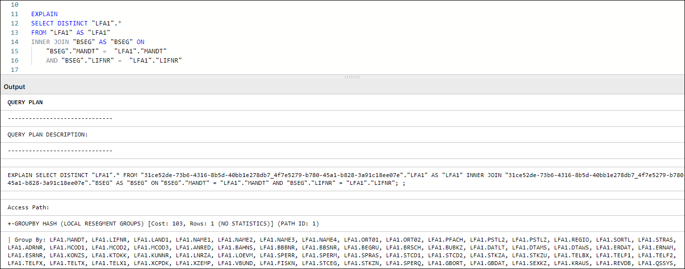
Figure 1: Query Plan Example in Vertica
The complexity of the query will determine the variety of information contained in the Query Plan. In most cases, our checks on query performance focus on specific areas as expanded in the following sections of the guide.
For use with tables containing 10,000 or more records
You should only create statistics for tables that have 10,000 records or more. The effort required to create statistics for tables with fewer than 10,000 is greater than the time saved by using them.
Table Statistics are analytical summaries of tables that assist the query optimizer in making better decisions on how to execute the tasks involved with the query. They provide information about the number of rows and column cardinality in the table.
In tasks such as SELECT, JOIN, GROUP BY, the plan will indicate whether a table has statistics available or not for the execution of query tasks.
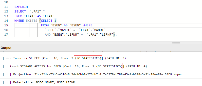
Figure 2: Example Query Plan showing NO STATISTICS for BSEG table
By default, Table Statistics are automatically updated for all raw tables extracted from the source system via Celonis Extractor (e.g. VBAK, EKKO, LIPS).
However, any temporary or other tables created and used in Transformations will not have table statistics refreshed by default. Missing Table Statistics will impact all downstream transformations that use the tables, as well as Data Model loading times in some cases. To ensure optimal performance, an ANALYZE_STATISTICS command should be executed when creating any table via Transformations.
Users can check which tables in their schema do not have Statistics refreshed by running the following query:
SELECT anchor_table_name AS TableName

FROM projections

WHERE has_statistics =FALSE ;
If this query returns any result, a SELECT ANALYZE_STATISTICS ('TABLE_NAME'); should be added in the transformation script that creates the respective table and database will gather table statistics when the query/transformation is executed.
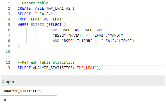
Figure 3: Example Table Creation & Table Statistics Refresh, with typical SQL Workbench output
In SQL, DISTINCT is a very useful command when needing to check or count distinct values in a field, or deduplicate records in smaller tables. While the use of DISTINCT in such cases is necessary, many users resort to DISTINCT (eg SELECT DISTINCT *) often times as a quick fix to remove duplicate records that result from the following scenarios:
Bad Data Quality: The extraction of the source table has quality issues that show up as duplicate records. These issues, if they exist, should be addressed at a source system/extraction level.
Use of DISTINCT to limit table population: A join is performed between two or more tables to limit the scope of the table content to only entries relating to records that exist in another table (e.g. AP_LFA1 Data model table is table LFA1 limited to Vendors who appear in AP Invoice Items).
In Vertica specifically, DISTINCT works as an implied GROUP BY, as can be seen in Figure 1. In that example, the GROUPBY HASH task has a significant cost proportionally to the total cost and is used to limit the LFA1 table population. In such cases, we suggest avoiding the use of DISTINCT and finding alternative ways to avoid the duplication caused by using JOIN to limit LFA1, and using WHERE EXISTS instead.
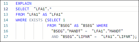
Figure 4: Example using WHERE EXISTS instead of JOIN + SELECT DISTINCT
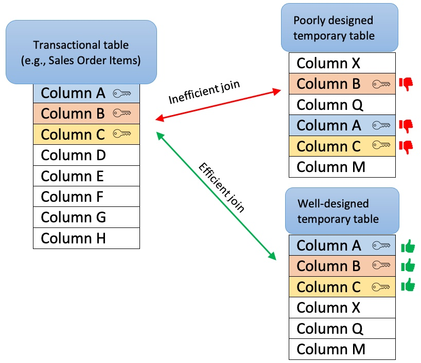
How do temporary join tables affect Transformation performance?
When creating temporary join tables, users should think about the purpose of the table and its relations with other tables (joins). In that respect, a well-designed temporary table:
Has a clear purpose, for example, to pre-process or join data, filter out irrelevant records, calculate certain columns that will be used later in transformations, etc. The sense of purpose should be validated, so as to confirm that the creation of temporary tables has a positive impact on overall performance.
Contains only necessary data (e.g. only really required columns and records).
Is sorted by the columns most often used for joins with other tables (e.g., MANDT, VBELN, POSNR). To ensure the proper sorting of the table, put those columns at the beginning of the create table statement or add an explicit ORDER BY clause at the end of the statement.
Doesn’t contain custom/calculated fields in the first column(s). As shown in the example below, the first columns should be the ones that are used for joins (key columns). If this is not the case, Vertica will have to perform additional operations (e.g. creating hash tables) while running the queries, which will extend the execution time.
In the example below, auxiliary table O2C_VBAK_VBAP is being defined with an improper column order. This in turn will cause the table to be sorted by the fields in the order they appear in the SELECT statement. The expected use case of this table involves joins on VBAK key fields (MANDT, VBELN, POSNR) which are not the fields that are part of the table sorting. In such a use case and with the definition of the table as seen on the left side, the joins to this table will not be performed optimally.
The correct definition for the table should have the table fields ordered initially with the table keys, then any other custom keys that may be used in joins, followed by calculated and other fields, as see on the script example on the right. This will ensure that the table is sorted by the fields that are used as condition joins and will result in a more efficient execution plan when joining to this table. In most cases, that would be a MERGE JOIN.
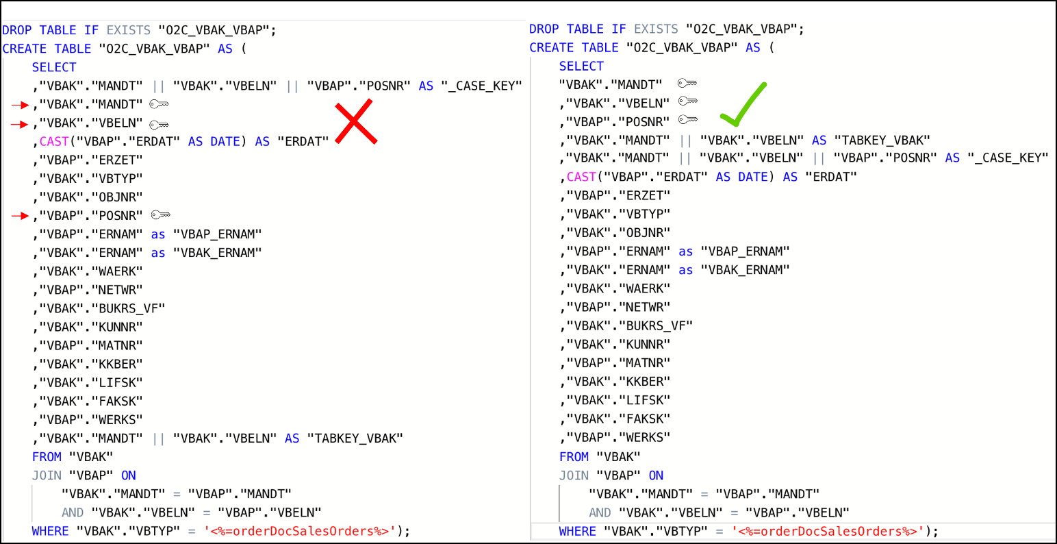
Figure 5: Example Scripts of poorly designed temporary table (left) vs well-designed temporary table (right)
Alternatively, an explicit ORDER BY can be used when creating a table in order to force a specific ordering of the new temporary join table.
Note
MERGE and HASH Joins
Vertica uses one of two algorithms when joining two tables:
Hash Join - If tables are not sorted on the join column(s), the optimizer chooses a hash join, which consumes more memory because Vertica has to build a sorted hash table in memory before the join. Using the hash join algorithm, Vertica picks one table (i.e. inner table) to build an in-memory hash table on the join column(s). If the table statistics are up to date, the smaller table will be picked as the inner table. In case statistics are not up to date or both tables are so large that neither fits into memory, the query might fail with the “Inner join does not fit in memory” message.
Merge Join - If both tables are pre-sorted on the join column(s), the optimizer chooses a merge join, which is faster and uses considerably fewer resources.

So which join type is appropriate?
In general, aim for a merge join whenever possible, especially when joining very large tables.
In reality, transformation queries often contain multiple table joins. So, it's rarely feasible to ensure that all tables are joined as a merge type because it requires tables to be presorted on join columns.
A merge join will always be more efficient and use considerably less memory than a hash join. But it's not necessarily faster. If the data set is very small, a hash join may process faster but this is very rare.
Alongside the creation of a well-designed temporary table, it is also essential to make sure that two tables are adequately joined by the entire join predicates (keys). For example, the MANDT (Client) column is often unduly excluded from join predicates which can have a very negative impact on query performance, ignoring potential MERGE JOIN even when both data sets are properly sorted, as seen in the following example:
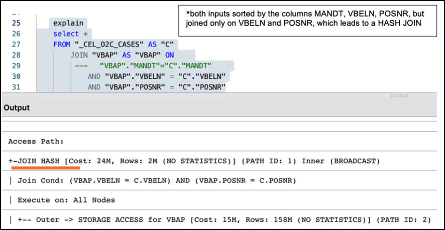
Figure 6: Example of Performance Impact between using partial and entire keys when joining tables
Note
What are Projections?
Unlike traditional databases that store data in tables, Vertica physically stores table data in projections. For every table, Vertica creates one or more physical projections. This is where the data is stored on disk, in a format optimized for query execution.
The projection created needs to be sorted by the columns most frequently used in subsequent joins (usually table keys), because the projection sorting acts like indexes do in Oracle SQL or SQL Server. The sorting of the underlying table projection is why users are encouraged to properly structure and sort their tables, as described in the section above.
Currently, two projections are used in Celonis Vertica Databases for extracted tables:
Auto-projection (super projection) created immediately on table creation. It includes all table columns and is sorted by the first 8 fields, at the order they are exported.
If the primary key is known (set up in the table extraction setting), Vertica creates additional projections sorted by and containing only the primary key fields. Such projections may be used by Vertica for JOIN or EXIST operations.
The performance of all queries that use temporary/auxiliary tables (i.e. all tables created during transformation) will heavily depend on the super-projection that is created by Vertica at the time of the table’s creation. By default, Vertica sorts the default super-projection by the first 8 columns as defined in the table definition script.
Additional read:
Using views instead of tables might negatively impact transformations and data model load performance. While a temporary table stores the result of the executed query, a view is a stored query statement that has to be executed every time it is invoked.
Aspect | View | Table |
|---|---|---|
When it is executed | During data model loads. | During transformations. |
Persistence | Is saved in memory. | Is persisted to storage. |
Life cycle | Resulting dataset is dropped after the query which called it no longer needs it. | Is dropped when a DROP TABLE statement is executed. |
When to use |
|
|
Common mistakes | Nested views – a query can call a view, which calls another view. This causes poor performance and a high risk of errors. | Poor design – the first columns of such tables should be primary/foreign keys in subsequent transformations (to promote merge joins over hash joins). |
Statistics | Views cannot have own statistics – query planner uses statistics of underlying tables. | Tables can (and should) have own statistics. |
Sorting | Do not have own sorting, uses sorting of underlying tables. | Can have own sorting – if sorted on columns used for joins, promotes more performant merge joins. |
All things considered, one should analyze the specific scenario, ideally, test both approaches and choose the one which is more performant in terms of total transformation and data model load time.
Implementing Staging Tables for Data Model
For every source table that is needed to be present in the Data Model (eg. VBAP), the standard approach is to define a table or view (e.g. O2C_VBAP), with all VBAP fields (VBAP raw data), as well as additional calculated/converted fields that will be needed for analyses (VBAP Transformed Data). In instances of large transactional tables such as VBAP, a user may face the following dilemma:
Define O2C_VBAP as a Table: The table will be loaded faster in the Data Model, but the Transformation defining it will be running longer than defining a view. APC consumption will also be increased, as all VBAP columns will need to be stored twice, once in the source table (VBAP) and another in the Data Model Table (O2C_VBAP).
Define O2C_VBAP as a View: The definition in the Transformation will only need seconds to run and there will not be an impact on APC. However, Data Model load runtimes will increase, as the view will need to be invoked and run and its resulting set will then need to be loaded in the Data Model.
While both scenarios above have their pros and cons, and some users may be satisfied with those based on their use case and data size, the most optimal way is to use both View and Table structures, to leverage the advantages of both, and balance savings in APC as well as reductions in overall runtime.
When defining the Staging Table, VBAP keys (MANDT, VBELN, POSNR) should be selected first. The statement should also include all the joins and functions required to define the Transformed Data fields (calculated fields). The users now have a table structure containing all additional fields for VBAP data model table, without having to store the rest of the original VBAP fields twice, which results in reduced APC consumption.
Subsequently, a data model view is created (e.g. O2C_VBAP), which joins the “raw data” table (i.e. VBAP) with the transformed data table (i.e. O2C_VBAP_STAGING). As the two tables (VBAP and Staging) are joined on keys and it is the only join taking place during the Data Model load, the materialization of the view is much more performant.
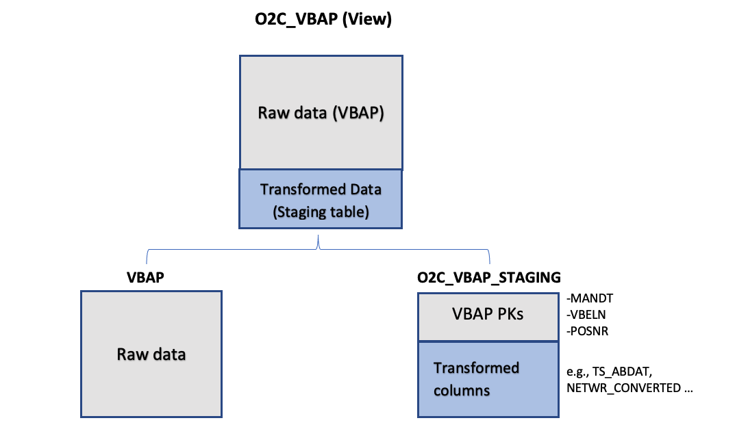 |
Figure 7: Leveraging Staging Tables in Data Model. In this example, View O2C_VBAP is based on a join between the existing source table (VBAP) and O2C_VBAP_STAGING table.
Important
A common problem with long running transformations and slow data model loads is due to missing statistics in Vertica. This issue can be resolved by adding the Vertica ANALYZE_STATISTICS statement directly in the SQL. For more information, refer to Vertica Transformations Optimization.
Example: Staging Table Definition (O2C_VBAP_STAGING):
CREATE TABLE "O2C_VBAP_STAGING" AS
(
        SELECT

        "VBAP"."MANDT", --key column
                "VBAP"."VBELN", --key column
                "VBAP"."POSNR", --key column
        CAST("VBAP"."ABDAT" AS DATE) AS "TS_ABDAT",
        IFNULL("MAKT"."MAKTX",'') AS "MATNR_TEXT",
        "VBAP_CURR_TMP"."NETWR_CONVERTED" AS "NETWR_CONVERTED",
        "TVRO"."TRAZTD"/240000 AS "ROUTE_IN_DAYS"
        FROM "VBAP" AS "VBAP"
        INNER JOIN "VBAK" ON
            "VBAK"."MANDT" = "VBAP"."MANDT"
                    AND "VBAK"."VBELN" = "VBAP"."VBELN"
                AND "VBAK"."VBTYP" = '<%=orderDocSalesOrders%>'
        LEFT JOIN "VBAP_CURR_TMP" AS "VBAP_CURR_TMP" ON
            "VBAP"."MANDT" = "VBAP_CURR_TMP"."MANDT"
                AND "VBAP"."VBELN" = "VBAP_CURR_TMP"."VBELN"
                AND "VBAP"."POSNR" = "VBAP_CURR_TMP"."POSNR"
                LEFT JOIN "MAKT" ON
                "VBAP"."MANDT" = "MAKT"."MANDT"
                        AND "VBAP"."MATNR" = "MAKT"."MATNR"
            AND "MAKT"."SPRAS" = '<%=primaryLanguageKey%>'
            LEFT JOIN "TVRO" AS "TVRO" ON
                        "VBAP"."MANDT" = "TVRO"."MANDT"
                        AND "VBAP"."ROUTE" = "TVRO"."ROUTE"
);
Example: Data Model View Definition (O2C_VBAP):
--In this view the only one join, between the raw table (VBAP) and the staging table (O2C_VBAP_STAGING) is performed. All other joins, required for calculation of the fields should be part of the STAGING_TABLE statement

CREATE VIEW "O2C_VBAP" AS (
        SELECT
        "VBAP".*,
                "VBAP_STAGING"."TS_ABDAT",
                "VBAP_STAGING"."MATNR_TEXT",
                "VBAP_STAGING"."TS_STDAT",
                "VBAP_STAGING"."NETWR_CONVERTED",
                "VBAP_STAGING"."ROUTE_IN_DAYS",
        FROM "VBAP" AS "VBAP"
        INNER JOIN "O2C_VBAP_STAGING" AS VBAP_STAGING ON
            "VBAP"."MANDT" = "VBAP_STAGING"."MANDT"
                    AND "VBAP"."VBELN" = "VBAP_STAGING"."VBELN"
                AND "VBAP"."POSNR" = "VBAP_STAGING"."POSNR"
);
Nested Views and Performance
In many cases, the use of nested views can affect performance, especially when used in Data Model views. While views are useful when wanting to run simple statements (such as SELECT) on a pre-defined result set, they should not be interchangeable with table structures in their usage. When dealing with transaction data (ie the larger data sets), we discourage users from performing transformation queries that join multiple views together, or using views in the definition of (Data Model or other) views, similar to the structure below:
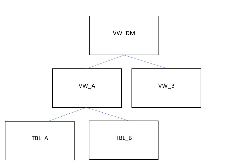 |
Figure 8: Example of Nested Views in a Data Model View Definition
In this example. View A is defined by a transformation that uses Tables A and B. View A is then joined to View B in the transformation that defines the Data Model View. When the Data Model View is invoked during the Data Model Load, VW_DM will have to be materialized at that stage, which includes running all the following tasks:
The transformation query that creates VW_A will be executed.
The transformation query that creates VW_B will be executed.
The transformation query that creates VW_DM will be executed.
The execution of all those steps/tasks together will greatly affect Data Model Load performance. In addition to that, any tasks that use views instead of tables, in our case the definition of VW_DM, will not be able to use projections, table sorting or table statistics, thus making the data model load execution even slower. This problem compounds as users add more view layers and more numbers of joins between views in order to reach their desired output.
In such cases, we strongly suggest the use of auxiliary/temporary tables in intermediary transformation steps, with their table statistics fully analyzed. Auxiliary tables can then be dropped as soon as they are no longer needed for further transformations. In our example above, Views VW_A and VW_B, as well as View VW_DM, should be created as tables instead, with VW_A and VW_B being dropped right after VW_DM is created.
When creating transformation queries, every choice has an impact on performance. Understanding the impact gives us the possibility to apply the best practices, avoid anti-patterns and improve overall query performance.
Every transformation (data preparation and cleaning) in the Celonis Event collection module is executed in the Vertica. For each query submitted to Vertica, the query optimizer assembles a query execution plan, a set of required operations for executing a given query.
When creating transformation queries, every choice has an impact on performance. Understanding the impact gives you the possibility to apply the best practices, avoid anti-patterns and improve overall query performance.
The following guidelines for improving overall query performance should be considered:
Check table statistics
Very easy to implement and significantly improve query performance
Automatically added for all raw tables after extraction
For each temporary table, statistics should be created explicitly by adding the SELECT ANALYZE_STATISTICS('TableName')
Check if all relevant tables have statistics by running the EXPLAIN statement
Check temporary (auxiliary) tables
Content - only necessary data, nothing more
Columns used for joins should be the first columns in create table statement (e.g. MANDT, VBELN, POSNR) or have an explicit ORDER BY clause at the end of the statement
Non-key, custom columns (e.g. Schema_id, source name, etc.) should not be placed at the beginning of the table (affects the sorting and later joins)
ANALYZE_STATISTICS ('TableName') statement added after the create table statement
Check the query statements validity
Avoid SELECT DISTINCT
Make sure that tables are joined properly (to avoid duplication / cartesian product)
Make sure that the entire key is used for joins (e.g., MANDT not ignored)
Join only necessary tables and check if all are really used
Revise the flow of logic, consider other approaches to achieve the same result
Reconsider view/ temp tables
Look for views with big complexity and try replacing them with a temp table (persisted results). It might affect APC and transformation time, but bring stability and overall faster transformation+data model load time
Consider implementing staging tables to enhance data model tables creation and loading
Table statistics are analytical summaries of tables that assist the query optimizer in making better decisions. They provide information about the number of rows or value cardinality in the table.
For tables extracted using Celonis extractor (i.e., “Raw” tables), statistics are automatically updated for each table after the extraction. For custom or temporary tables created within transformations, it is necessary to create statistics explicitly.
To do that, add on the SELECT ANALYZE_STATISTICS ('TABLE_NAME'); after each "Create table" statement, and database will gather statistics in the background.
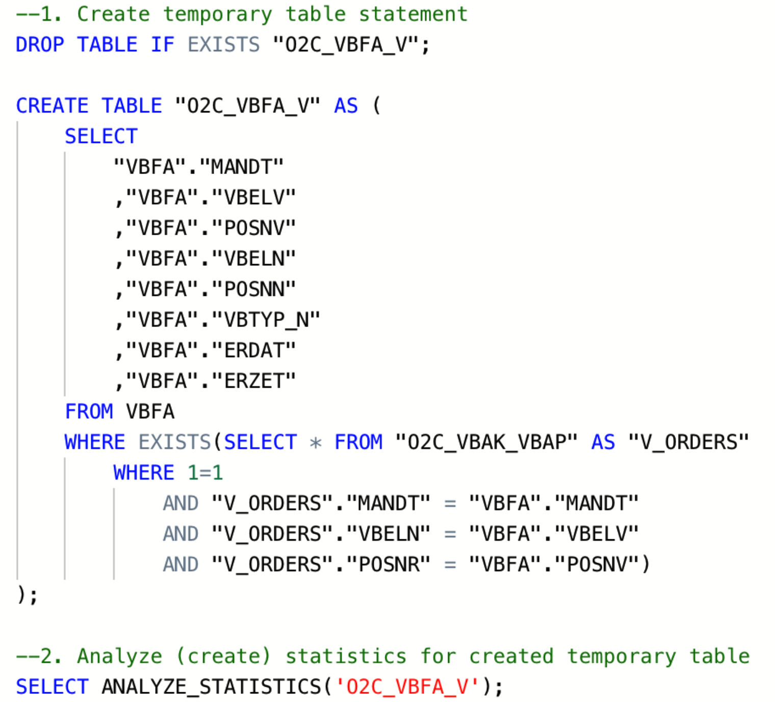 |
Image 1: Example statements for creation of temporary table and statistics
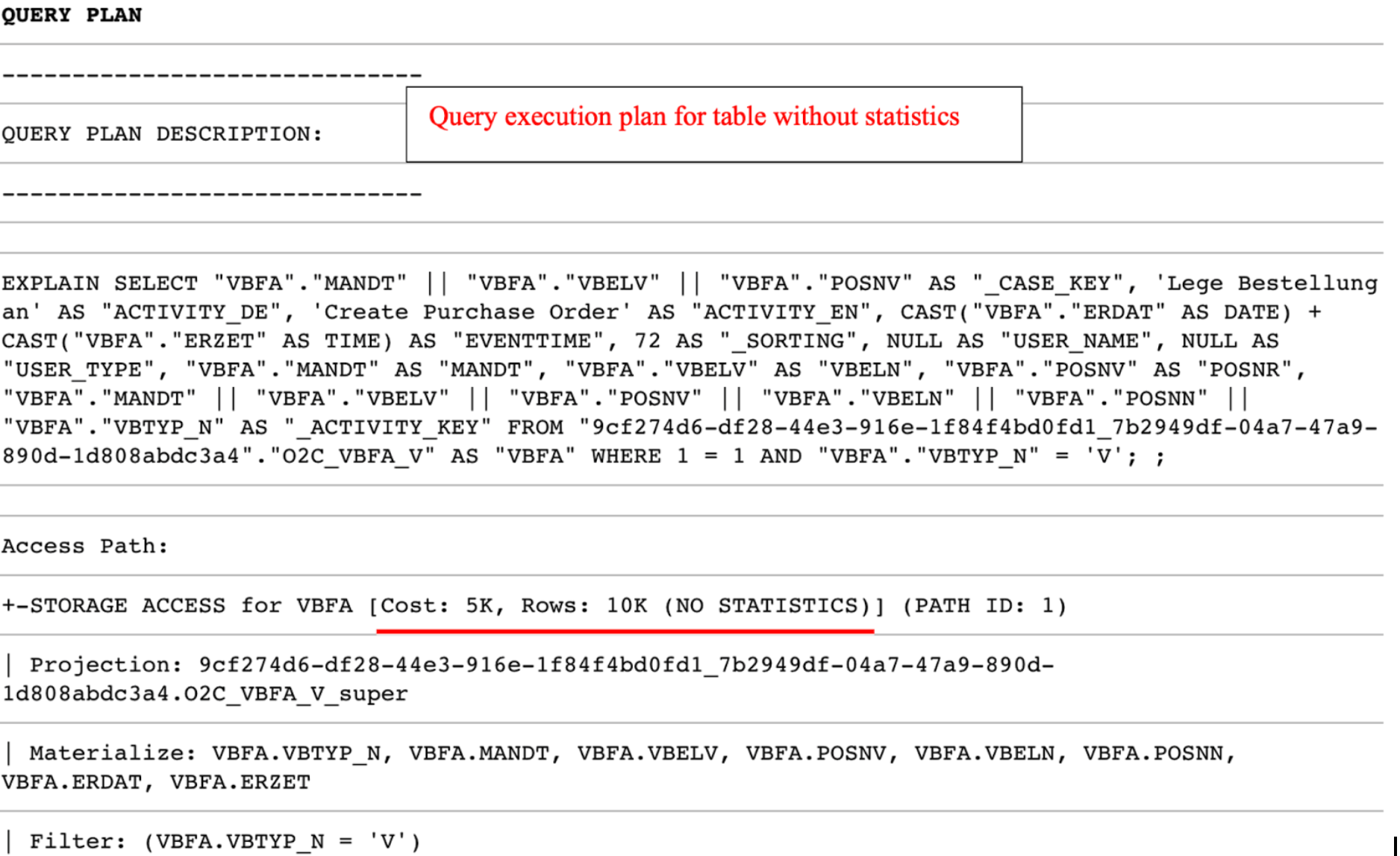
One of the ways to check if all tables in certain queries contain statistics is by reading the query execution plan (EXPLAIN function). If there is “NO STATISTICS” next to a table name, the given table has no statistics. In that case, you need to add the SELECT ANALYZE_STATISTICS (‘TABLE_NAME’); statement after creating this table. Once you ran the statement and generated statistics you can check again using the EXPLAIN function.
Access Path: |
+-STORAGE ACCESS for VBFA [Cost: 798, Rows: 7K (NO STATISTICS)] (PATH ID: 1) |
Example of a query plan where a table “VBFA” does not have statistics
Two scenarios with corresponding query costs are shown in the screenshot below. In the first scenario, the O2C_VBFA_V temporary table is created without statistics, whereas in the second one, statistics have been created for the same table.
 |
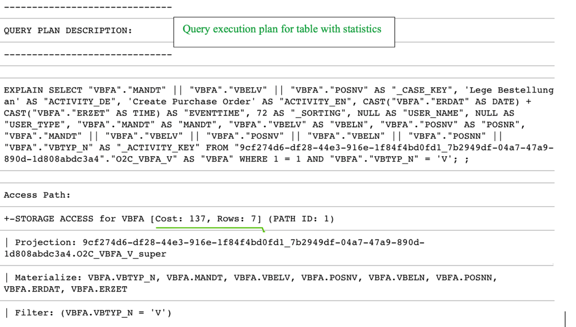 |
Another way to get a list of tables without statistics is by running the following query:
Check for tables without gathered tables statistics
SELECT anchor_table_name AS TableName FROM projections WHERE has_statistics =FALSE ;
If this query returns any result, you should go to transformation script that creates the respective table and add the SELECT ANALYZE_STATISTICS ('TABLE_NAME'); after the "Create table" statement, save the transformation, and database will gather statistics in the background.
Note
Table statistics are crucial for query execution plans with HASH JOINS. They enable the query optimizer to choose the smaller table to produce the HASH table (instead of the bigger one). In most scenarios, this prevents the “inner join did not fit into memory” error.
Table statistics additional read
The temporary, or auxiliary table in this article refers to any table that is created in addition to tables extracted from the source system (raw tables). Those temporary tables (e.g. TMP_VBAP_VBAK, TMP_CDPOS_CDHDR, etc.) are created in the transformation phase.
When creating temporary tables, one should think about the purpose of the table and its relations with other tables (joins). A well-designed temporary table:
Has a clear purpose, for example, to pre-process or join data, filter out irrelevant records, calculate certain columns that will be used later in transformations, etc. The sense of purpose should be validated, to confirm that the creation of temporary tables has a positive impact on overall performance.
Contains only necessary data (e.g. only really required columns and records)
Is sorted by the columns most often used for joins with other tables (e.g., MANDT, VBELN, POSNR). To ensure that, put those columns at the beginning of the create table statement or add an explicit ORDER BY clause at the end of the statement.
Doesn’t contain custom/calculated fields in the first columns. The first columns should be the ones that are used for joins (key columns). If this is not the case, Vertica will have to perform additional operations while running the queries, which will extend execution time.
Contains the Update statistics statement after the create table statement
 |
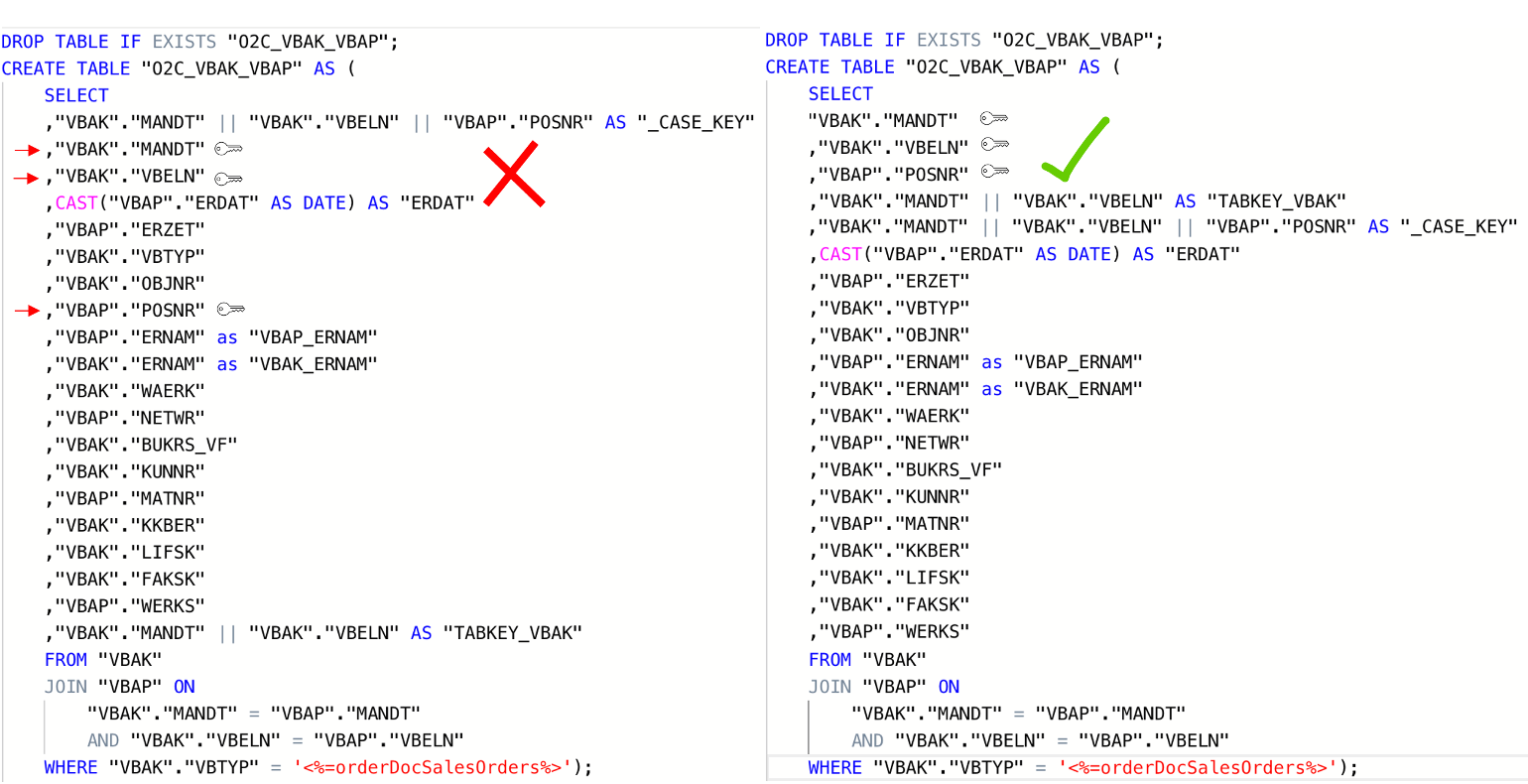 |
Image 2: Inadequately designed temporary table (left) vs Well-designed temporary table (right)
Table Sorting
If the table is not explicitly sorted during the creation statement (by adding an “ORDER BY”), the table (projection) will by default be sorted by the first eight columns in the order defined by the creation statement.
MERGE and HASH joins
Vertica uses one of two algorithms when joining two tables:
Merge join- If both tables are pre-sorted on the join column(s), the optimizer chooses a merge join, which is faster and uses considerably fewer resources.
Hash join - If tables are not sorted on the join column(s), the optimizer chooses a hash join, which consumes more memory because Vertica has to build a sorted hash table in memory before the join. Using the hash join algorithm, Vertica picks one table (i.e. inner table) to build an in-memory hash table on the join column(s). If the table statistics are up to date, the smaller table will be picked as the inner table. In case statistics are not up to date or both tables are so large that neither fits into memory, the query might fail with the “Inner join does not fit in memory” message.
Vertica Projections
Unlike traditional databases that store data in tables, Vertica physically stores table data in projections. For every table, Vertica creates one or more physical projections. This is where the data is stored on disk, in a format optimized for query execution.
Currently, two projections are used in Celonis Platform:
Auto-projection (super projection) created immediately on table creation. It includes all table columns,
If the primary key is known (set up in the table extraction setting), Vertica creates additional projection based on it.
Additional information:
A key difference between a hash join and a merge join lies in how each operation handles memory and sorting:
Hash join: Typically loads one side of the join (often the smaller table or a subset of rows) into memory. This can cause memory pressure and potentially degrade performance for other queries running concurrently.
Merge join: Requires both input tables to be sorted on the join columns. It often performs better than a hash join - especially when joining very large tables, because it avoids the overhead of loading large datasets into memory.
Why force a merge join?
If you examine your query execution plan and notice that two large tables are joined using a hash join, you may be able to improve performance by sorting the data on the join columns so that the optimizer can use a merge join instead. In many cases, forcing a merge join yields better overall performance, but it is advisable to test this approach for your particular workload to confirm any benefits.
Example scenario for a merge join
Suppose your first table is already physically sorted on the ID column (perhaps due to its projection or index), but the second table does not have a compatible projection on Header_ID. Because the second table is not sorted, the optimizer defaults to a hash join.
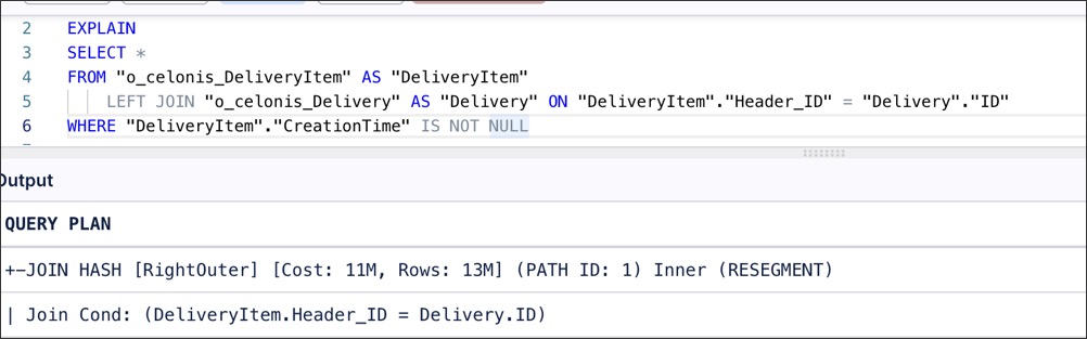 |
However, if you wrap the second table in a subquery that explicitly sorts by Header_ID, the optimizer will detect that both inputs are sorted and switch to a merge join.
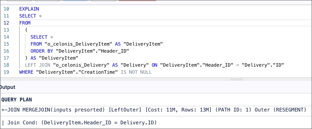 |
Impact under high load
The advantage of using a merge join becomes more pronounced when multiple queries or transformations run concurrently. A large hash join can occupy a significant portion of available memory, slowing down other queries. In contrast, a merge join typically uses less memory for large datasets, resulting in more consistent performance across all running queries.
Alongside the creation of a well-designed temporary table, it is essential to make sure that two tables are adequately joined by the entire join predicates (keys). For example, the MANDT (Client) column is often unduly excluded from join predicates which can have a very negative impact on query performance, ignoring potential MERGE JOIN even when both data sets are properly sorted.
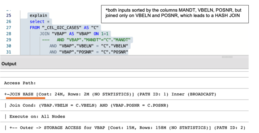 |
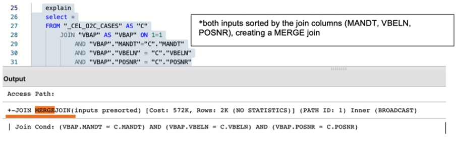 |
Image 3: The impact of using the partial and entire keys when joining two tables
Users often join the same table more than once within one query. Even if the join is identical, it is executed multiple times, leading to increased execution time and risk of error. For example, while creating the Data Model table O2C_VBAP, beside the main case table (VBAP), temporary tables with essentially identical records are often needlessly joined (e.g TMP_VBAP_VBAK, _CEL_O2C_CASES). Usually, the idea behind those redundant joins is filtering or adding some calculated columns (e.g., converted net value).
Best practice:
Evaluate the business needs and only use necessary tables and columns
Revise the flow of logic and consider alternatives to achieve the same (e.g. by using smaller tables such as original (raw tables)
In situations where joining tables with very similar data (e.g. VBAP with TMP_VBAP_VBAK) is unavoidable, make sure that join is ofMERGEkind.
Using views instead of tables might negatively impact transformations and data model load performance.While a temporary table stores the result of the executed query, a view is a stored query statement that is being executed only when invoked.
Each option has advantages and disadvantages and making the right choice highly depends on the table size and structure and query complexity. While replacing a table with a view reduces required storage (APC), it could negatively affect the overall performance and significantly increase total execution time. If the query contains complex logic in terms of types of joins and conditions, the best practice will most likely be the creation of a well-designed temporary table, by fully taking into account previously described recommendations. If the query simply selects all the records from some raw table (e.g. VBAP) or applies simple conditions, a view might be a more reasonable choice. All things considered, one should analyze the specific scenario, ideally, test both approaches and choose the one which is more performant in terms of total transformation and data model load time.
5.1 Implement staging tables for Data model loading
For tables that are being loaded into the Data Model, the best balance in terms of required storage and performance of the entire pipeline is to combine the temporary table (i.e. Staging_table) with a view, as shown on the diagram below.
The statement (example below) that creates the staging table should include all the joins and functions required to calculate or reformat the column values. The staging table should contain only the primary keys and calculated/derived columns.
Subsequently, a data model view is created (e.g. O2C_VBAP), which joins the “raw data” table (i.e. VBAP) with the transformed data table (i.e. O2C_VBAP_STAGING). This approach allows us to achieve better performance without significantly affecting the APC.
Staging table statement example
CREATE TABLE "O2C_VBAP_STAGING" AS
(
        SELECT

        "VBAP"."MANDT", --key column
                "VBAP"."VBELN", --key column
                "VBAP"."POSNR", --key column
        CAST("VBAP"."ABDAT" AS DATE) AS "TS_ABDAT",
        IFNULL("MAKT"."MAKTX",'') AS "MATNR_TEXT",
        "VBAP_CURR_TMP"."NETWR_CONVERTED" AS "NETWR_CONVERTED",
        "TVRO"."TRAZTD"/240000 AS "ROUTE_IN_DAYS"
        FROM "VBAP" AS "VBAP"
        INNER JOIN "VBAK" ON 1=1
            AND "VBAK"."MANDT" = "VBAP"."MANDT"
                    AND "VBAK"."VBELN" = "VBAP"."VBELN"
                AND "VBAK"."VBTYP" = '<%=orderDocSalesOrders%>'
        LEFT JOIN "VBAP_CURR_TMP" AS "VBAP_CURR_TMP" ON 1=1
            AND "VBAP"."MANDT" = "VBAP_CURR_TMP"."MANDT"
                AND "VBAP"."VBELN" = "VBAP_CURR_TMP"."VBELN"
                AND "VBAP"."POSNR" = "VBAP_CURR_TMP"."POSNR"
                LEFT JOIN "MAKT" ON 1=1
                AND "VBAP"."MANDT" = "MAKT"."MANDT"
                        AND "VBAP"."MATNR" = "MAKT"."MATNR"
            AND "MAKT"."SPRAS" = '<%=primaryLanguageKey%>'
            LEFT JOIN "TVRO" AS "TVRO" ON 1=1
                        AND "VBAP"."MANDT" = "TVRO"."MANDT"
                        AND "VBAP"."ROUTE" = "TVRO"."ROUTE"
);
Data Model view statement example
--In this view the only one join, between the raw table (VBAP) and the staging table (O2C_VBAP_STAGING) is performed. All other joins, required for calculation of the fields should be part of the STAGING_TABLE statement

CREATE VIEW "O2C_VBAP" AS (
        SELECT
        "VBAP".*,
                "VBAP_STAGING"."TS_ABDAT",
                "VBAP_STAGING"."MATNR_TEXT",
                "VBAP_STAGING"."TS_STDAT",
                "VBAP_STAGING"."NETWR_CONVERTED",
                "VBAP_STAGING"."ROUTE_IN_DAYS",
        FROM "VBAP" AS "VBAP"
        INNER JOIN "O2C_VBAP_STAGING" AS VBAP_STAGING ON 1=1
            AND "VBAP"."MANDT" = "VBAP_STAGING"."MANDT"
                    AND "VBAP"."VBELN" = "VBAP_STAGING"."VBELN"
                AND "VBAP"."POSNR" = "VBAP_STAGING"."POSNR"
);